
Spatial Genetics - Landscape Ecology - Wildlife Conservation


In spatial genetic correlative analyses, as soon as pairwise aggregates are associated with more than one distance measure, that is when computing inter-individual genetic distances with more than one sampled genotype per aggregate (n > 1) rather than interpopulation genetic distances based of allelic frequencies, Mantel tests are to be performed with restricted permutations, as pseudo-replication issues may arise when clumped genotypes are considered independent (Prunier et al. 2013): in this case, permuted objects are the p blocks of n individuals, rather than the n individuals.
The following Matlab script can be used to perform simple and partial Mantel tests with standard or restricted permutations, depending on input data :
This is the version 2.0 of the script. You now have to specify whether you intend to perform a Mantel test with classical ('c') or with restricted ('r') permutations. It prevents issues due to the spatial alignment of sampling points when using classical permutations. You can also choose to perform one-tailed or two-tailed Mantel tests.
Please, contact me by email for any trouble, remarks or suggestions !
This is the R-version of Tool #1, now allowing MRDM (Multiple Regression on Distance Matrices) rather than (partial) Mantel test only :
Please, contact me by email for any trouble, remarks or suggestions !
Non-directional Mantel autocorrelograms may provide an insightful description of spatial patterns of genetic similarity among aggregates, especially when many aggregates are sampled across the study area (Prunier et al. 2013). With only a few sampled individuals per aggregate (but many prospected aggregates), Mantel correlograms are to be performed with restricted permutations.
The following Matlab script can be used to perform spatial autocorrelation analyses through non-directional Mantel correlograms with standard or restricted permutations (depending on input data) :
This is the version 2.0 of the script. You now have to specify whether you intend to perform a Mantel test with classical ('c') or with restricted ('r') permutations. It prevents issues due to the spatial alignment of sampling points when using classical permutations.
Please, contact me by email for any trouble, remarks or suggestions ! Many thanks to Dr J. Galarza for feedback on this script !
The following figure shows an example of plots you may get when using this script (here, spatial autocorrelation analysis in 40 aggregates of 5 individuals each). Genetic data were simulated in CDPOP (Landguth & Cushman 2010)
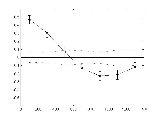
Non-directional Mantel autocorrelograms with restricted permutations and boostrap resampling. Error bars bound the 95% confidence interval about r (y-axis) as determined by bootstrap resampling. Upper and lower confidence limits (dotted line) bound the 95% confidence interval about r under the null hypothesis of no spatial structure. Black circles indicate a significant Mantel correlation value at alpha=5%.
CDpop (Landguth & Cushman 2010) is a well-known spatially explicit, individual-based population genetics tool that simulates birth, death, mating and dispersal of individuals in complex landscape as probabilistic functions of movement costs among sampling locations.
Depending on input parameters, a thorough understanding of simulated processes and resulting gene flow is of crude importance for an accurate use of CDpop.
The following R and Matlab scripts are based on provided individual ID in CDpop format output grids. It computes the mean number of interpopulation individual exchanges per generation and provides a summary matrix in .txt format.
The matrix allows a quick and informative overview of effective connectivity among populations for each CDpop run. Diagonal elements stand for internal recruitment, e.g. the mean number of non-immigrant individuals per generation.
Matlab script : CDpopinterpopExchange.m. This is the version 3.0 of the script, compatible with CDPOP v.1.2.18, and easily implemented in a loop.
R script : CDpopinterpopExchange.R
Please, contact me by email for any trouble, remarks or suggestions !
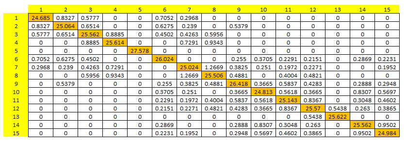
An output matrix providing the mean number of individual exchanges among 15 populations (N=30) per generation. Diagonal elements (in orange) correspond to the mean internal recruitment per population and per generation.
Commonality analysis (CA) is a detailed variance-partitioning procedure that can be used to deal with nonindependence among spatial predictors. By decomposing model fit indices into unique and common (or shared) variance components, CA allows identifying the location and magnitude of multicollinearity, revealing spurious correlations and thus thoroughly improving the interpretation of multivariate regressions (Prunier et al. 2015)
The following R and Rstudio scripts can be used to perform CA in both Multivariate Regression on Distance Matrices (MRDM) and Logistic Regressions on Distance Matrices (LRDM). These scripts allow visually investigating the normality of the dependent variable, choosing between MRDM and LRDM accordingly, performing adequate bootstrapping (taking into account the non-independence of pairwise data), and getting insightful numerical and graphical outputs. Note that both scripts are identical except for the preparation of graphs, the procedure being slightly different depending on the platform you use.
CAonDM stands for Commonality analyses on Distance Matrices.
You will find below some graphical outputs you can get with these scripts (Here, using dataset 1 from Prunier et al. 2015).
This new version (v0.4) of scripts provides additional graphical and numerical outputs (notably, structures coefficients and normality tests of residuals) ! Furthermore, input data can be either an R-list of pairwise matrices or a dataframe of linearized matrices !
Please, contact me by email for any trouble, remarks or suggestions !
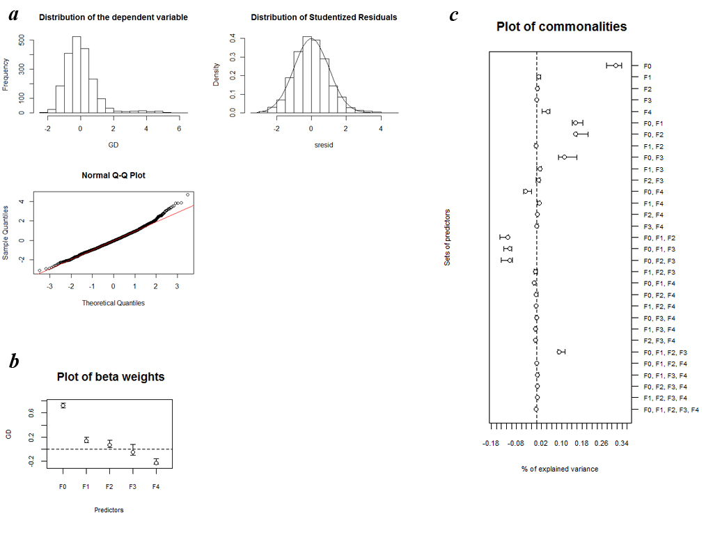
a) Distribution of the dependent variable, histogram and normal Q–Q plot of studentized residuals resulting from MRDM on quantitative datas.
b) Plot of β weights with 95% confidence intervals computed on the basis of 1000 replicates with a random removal of 10% of all 64 considered populations.
c) Plot of commonalities with 95% confidence intervals computed on the basis of 1000 replicates with a random removal of 10% of all 64 considered populations.
The following Rstudio script can be used to perform classical CA in both Linear and Logistic regressions, that is, using point data in a R-dataframe (in which each column stands for a specific vector), rather than pairwise matrices in a R-list (see Tools #5). They provide exactly the same outputs as Tools #5.
CAonV stands for Commonality analyses on Vector data.
This new version (v0.6) of scripts provides additional graphical and numerical outputs (notably, structures coefficients and normality tests of residuals) !
Please, contact me by email for any trouble, remarks or suggestions !
The following R functions allow the application of the permutation-based d-sep test, clustering-based path analysis, permutation-based path analysis and a parametric bootstrap procedure dedicated to the handling of pairwise matrices in path analysis, as described in Fourtune et al. 2018.
PAonDM stands for PAth Analyses on Distance Matrices.
Please, contact me or Lisa Fourtune by email for any trouble, remarks or suggestions !
Macdonald et al. (Ecol. Lett., 21, 2018, 207–216; doi: 10.1111/ele.12883) proposed an analytical framework for identifying evolutionary processes underlying trait-environment relationships (TER) observed in natural populations. It is based on the visual inspection of the graphical distribution of two summary statistics (β-weights Benv and Bint; see Figure 1 in Macdonald et al. 2018) that are also used to compute another summary statistic (L) described as an index of local adaptation. We proposed an expanded and refined framework based on simulations and bootstrap-based approaches.To make the interpretation of L, Benv and Bint more objective, we designed a bootstrap procedure to estimate 95% confidence intervals (CIs), and hence to take into account the uncertainty associated with each statistic. This refined approach, described in Prunier and Blanchet (2018), allows directly inferring processes underlying each TER independently, even when a single trait and single environmental variable are considered.
The R script BenvBintBootstrap.R can be used to implement the expanded Macdonald's framework. It may be used to compute Benv and Bint β weights, RSint structure coefficients, as well 95% CI about Benv and Bint as obtained from bootstrap.
The R script BenvBintBootstrapPlot.R can be used to plot outputs from the BenvBintBoostrap.R function as in Prunier and Blanchet (2018).
The R script InteractionPlot.R can be used to get both a fan-representation and a surface-representation of any first-order interaction.
You will find below some graphical outputs you can get with these scripts, here using the Macdonald’s empirical dataset revisited.
Please, contact me by email for any trouble, remarks or suggestions !
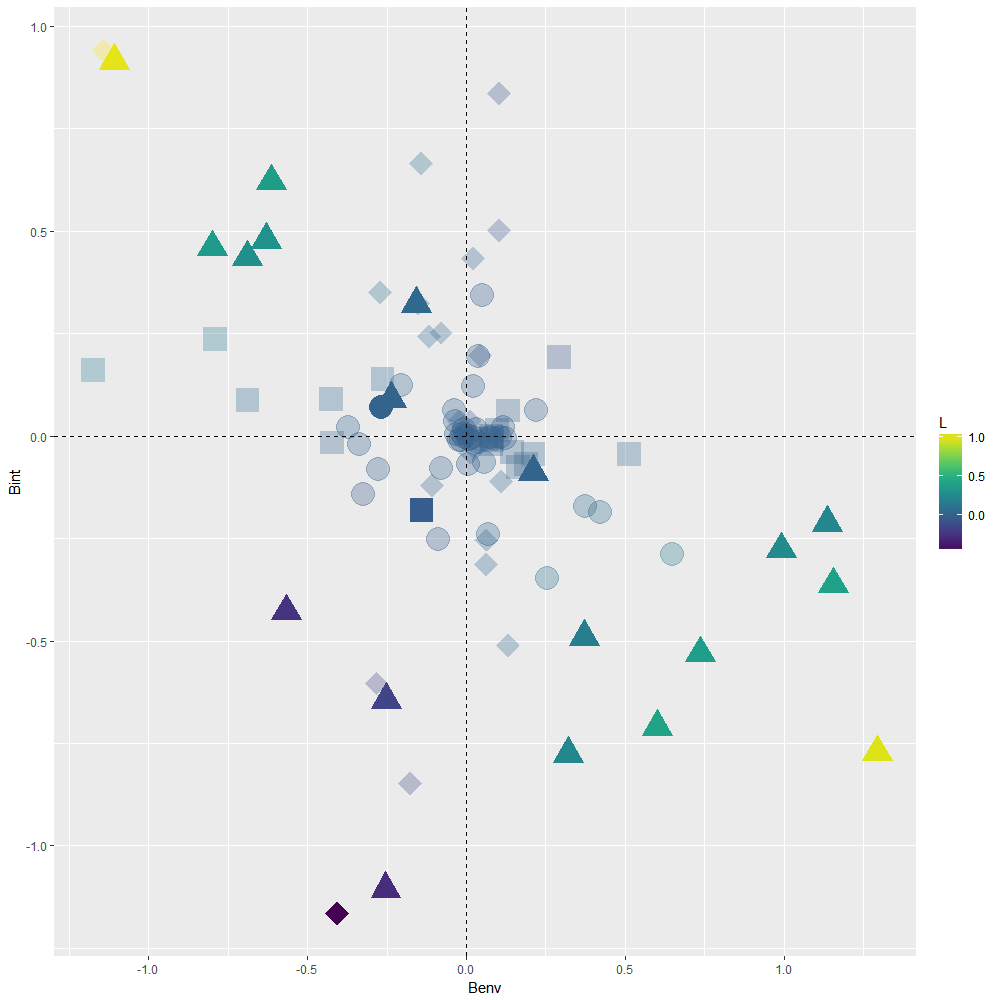
Scatterplot showing the results of 99 linear nested mixed effect models run to assess the putative driver of each TER in Macdonald et al. Symbols indicate whether a TER was found to be null (circles), driven by plasticity (squares) or driven by local adaptation (triangles) while taking uncertainty in the model estimates into account. Situations where Bint is non-null but Benv is null (diamonds) indicate that TER does not exist at intermediate levels of connectivity but does exist at low/high levels of connectivity, which may indicate that (mal)adaptation may covary non-linearly with connectivity . A solution to interpret ongoing processes in such situations is to plot predicted trait values obtained from the fitted model against explanatory variables (see InteractionPlot.R script). Colors indicate values for the L index of local adaptation. Faded colors indicate that the L index was not different from 0 according to 95% CI.
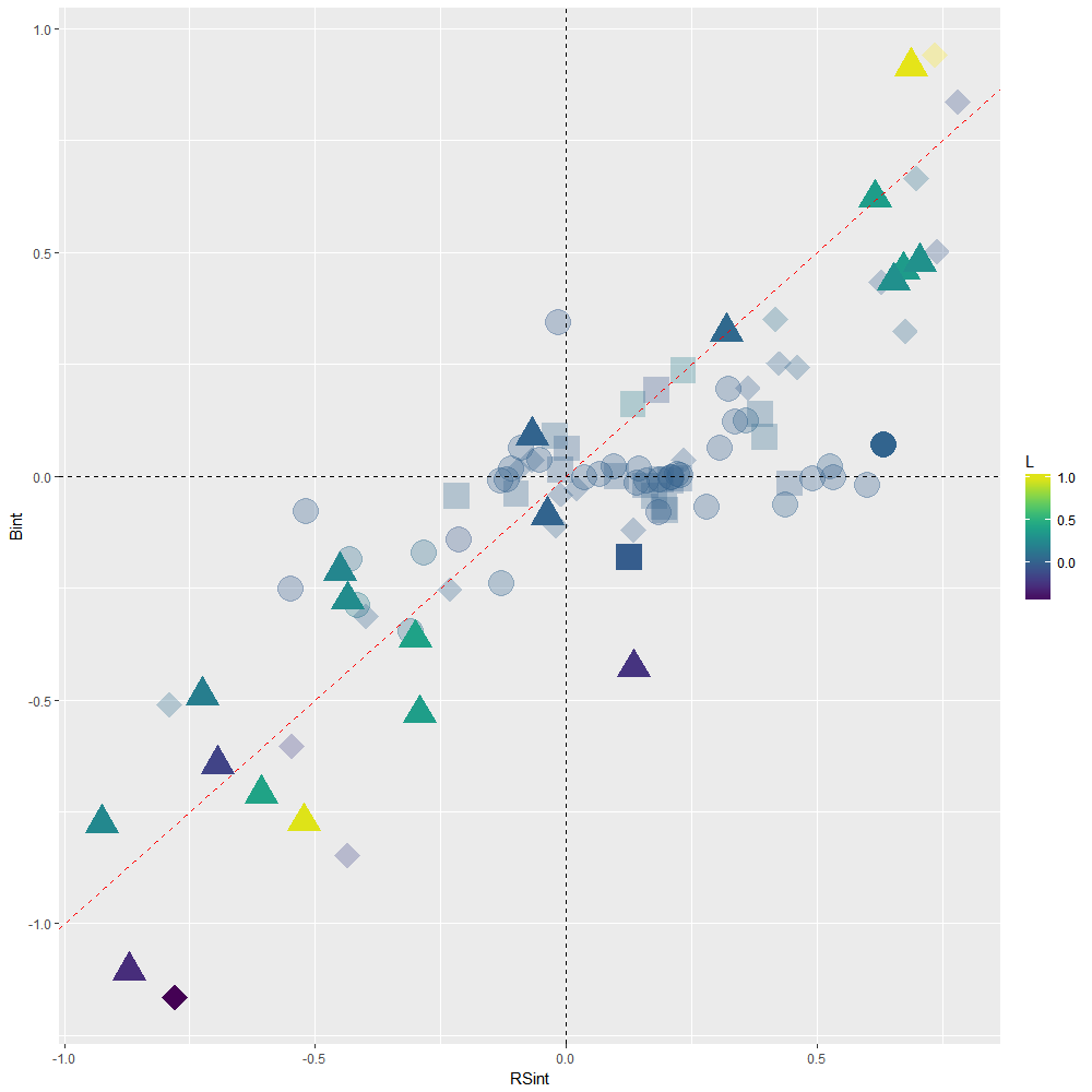
Scatterplot showing the distortion in Bint estimates due to multicollinearity, when compared to structure coefficients RSint. In absence of collinearity, Bint and RSint are supposed to be similar and corresponding TERs to line up along the red dashed 1:1 slope. Severe distortion (sign reversal) occurs within upper left and lower right quadrants, and concern 36 out of 99 TERs in Macdonald et al.’s dataset. These 36 TERs are therefore to be disregarded.
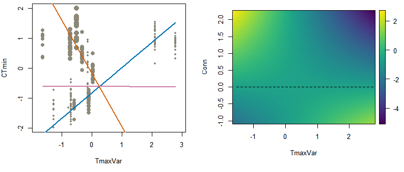
Panels a and b represent the CTmin ~ Tmaxvar TER as computed from a linear nested mixed effect models using Macdonald et al.’s dataset. Panel a shows a “fan representation” of the interaction (following Aiken et al. 1991), with predicted values computed at three different and contrasted levels of connectivity, that is, for minimal (“Low”, blue line), null (“Intermediate”, pink line) and maximal (“High”, orange line) values of connectivity. Grey points represent the observed positions of the trait values along the environmental gradient, the size of each point being proportional to the corresponding level of connectivity. Panel b shows a continuous representation of the interaction, with predicted values computed across all possible values of connectivity (the black dashed line indicating intermediate level of conectivity)and plotted as a colored surface in the Environment-Connectivity space. The TER at intermediate level of connectivity was null (according to 95% CI), but investigating TER at low and high levels of connectivity indicated that it was eroded by gene flow.
The following Rstudio script can be used to compute the Findex, a standardized genetic index of fragmentation allowing an absolute and independent assessment of the individual impacts of obstacles on functional connectivity. Briefly, the Findex is computed as the standardized ratio (expressed as a percentage) between the observed genetic differentiation between pairs of populations located on either side of an aquatic or a terrestrial obstacle and the genetic differentiation expected if this obstacle completely prevented gene flow. The expected genetic differentiation is predicted from a RandomForest algorithm trained on numerous simulations taking into account both the age of the barrier (expressed in number of generations elapsed since barrier creation) and the effective size of the targeted populations (based on expected heterozygosity as a proxy). See the bioRxiv preprint Prunier et al. (2019) for a complete description.
The computation of the Findex is automated in the user-friendly FINDEX() R-function (see R-walkthrough). The function is embedded within the FINDEXpackage.rda file. This .rda file also contains all RandomForest predictions required to compute the Findex. Users are invited to download this .rda file within their working directory, and to load/install required R-libraries (adegenet, randomForest, mmod, lme4 and reshape2) before running the FINDEX() R-function.
Illustration files are provided in the form of a compressed zip-file containing a parameter file (Prunier2018_illustration.txt) as well as two genepop files from Prunier et al. 2018 (Phoxinus.gen and Gobio.gen) that can be used to test the FINDEX() R-function.
Illustration files from Prunier et al. 2018
All these files are also available on Figshare.
You will find below the flowchart explaining how the Findex is computed, as well as a graphical output you can get with the FINDEX() R-function using illustration files from Prunier et al. 2018.
Please, contact me by email for any trouble, remarks or suggestions !
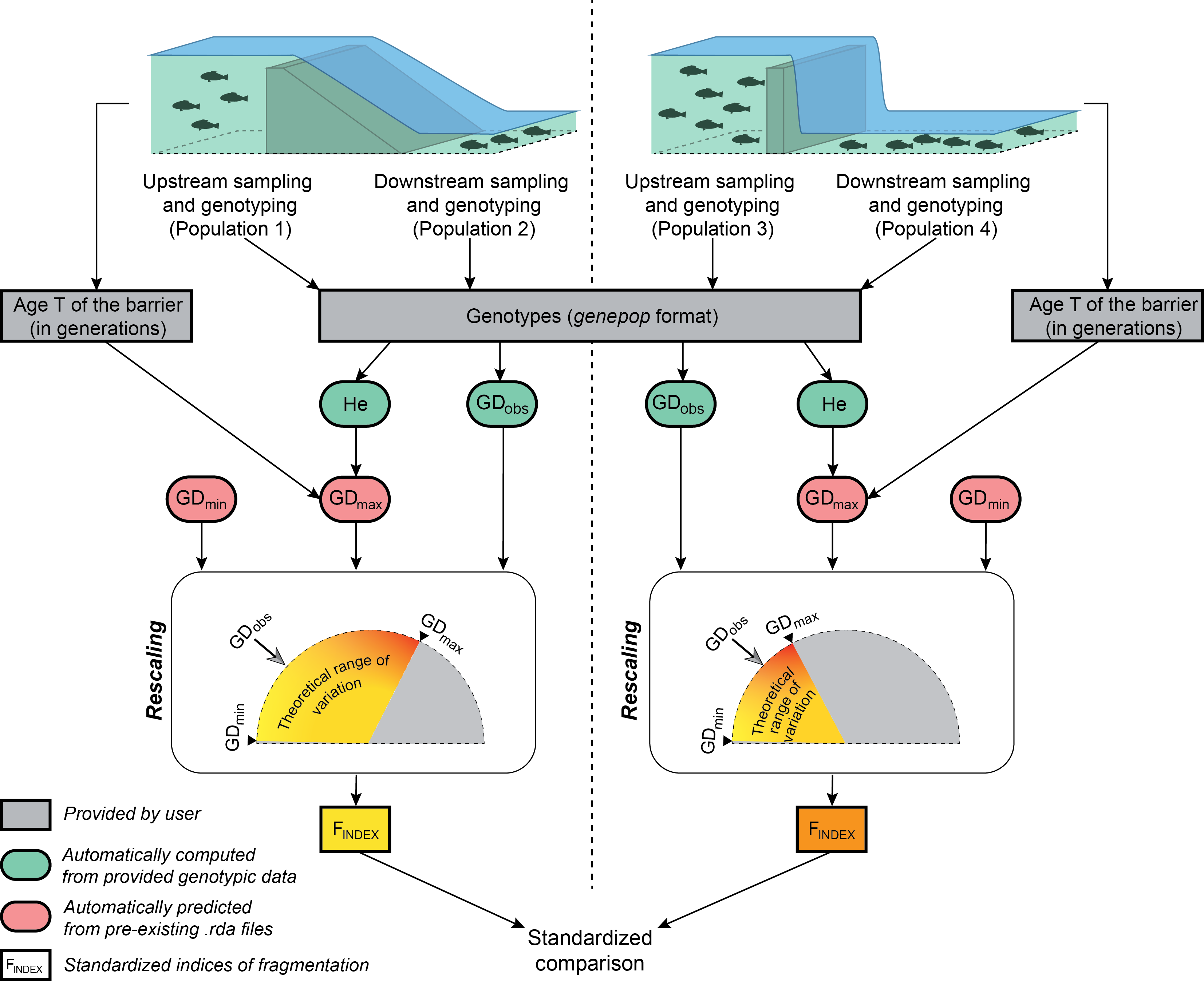
Flowchart illustrating the major steps in calculating the genetic index of frgmentation for two independent obstacles. After the sampling of populations located at the immediate upstream and downstream vicinity of each obstacle, users only have to provide a file of genotypes in the genepop format and a file of parameters indicating, for each obstacle, the names of the sampled populations and the number T of generations elapsed since the creation of the obstacle. Observed measures of genetic differentiation GDobs and mean expected heterozygosity He are automatically computed from provided genotypic data. GDmin and GDmax values, both delimiting the theoretical range of variation of GDobs, are automatically predicted from pre-existing .rda file, GDmax values depending on both He and T. The computation of the Findex basically amounts to rescaling GDobs within its theoretical range, thus allowing standardized comparisons of the permeability of various obstacles, whatever their age, the considered species or the effective size of sampled populations.
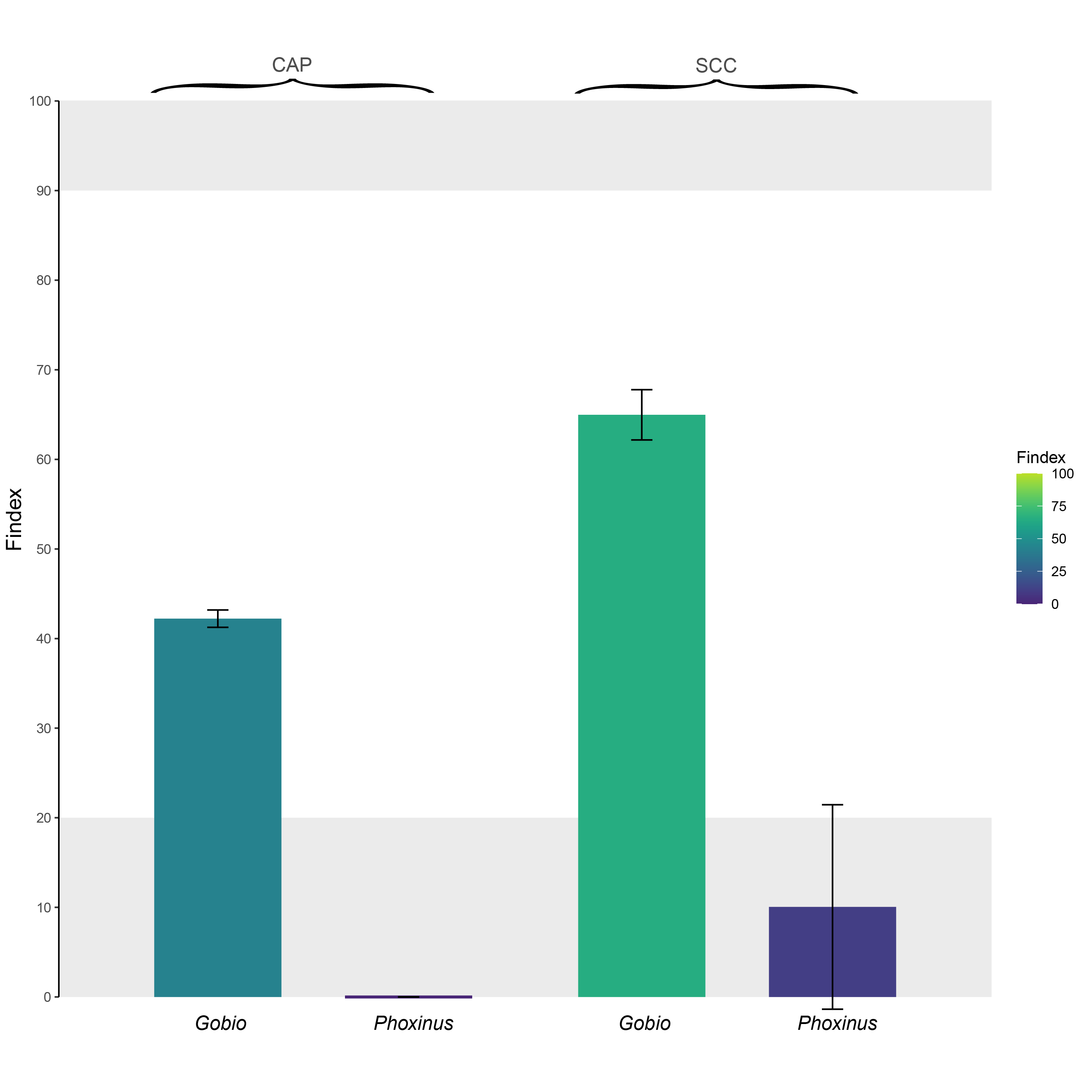
For each monitored species (Gobio: Gobio occitaniae; Phoxinus: Phoxinus phoxinus), Findex values for two weirs (CAP and SCC) selected from Prunier et al. 2018. These two weirs act as barriers to gene flow in Gobio occitaniae (Findex > 20 %), but not in Phoxinus phoxinus (Findex lower than 20 %). In the case of Gobio occitaniae, the Findex also allows ranking the obstacles from the most problematic (SCC; Cindex ~ 65 %) to the least problematic (CAP; Cindex ~ 42 %) in terms of fragmentation.
The following R function allows estimating the barrier effect of any linear feature based on recapture data, as described in Remon et al. 2018.
NEFbarrDetect stands for Negative Exponantial Function Barrier Detection.
Please, contact me or Jonathan Remon by email for any trouble, remarks or suggestions !